Microsoft products are generally MUCH more powerful than people realize.. probably because the advanced functions are not taught to us in high school and we never have another chance to realize the programs' full potential unless we happen to be trained in a job or do personal research on it (as I have). Now, what I am about to teach you doesn't require a lot of prior Excel knowledge and you don't need advanced skills to do this. But your outcome will be a powerful, useful little spreadsheet that you built on your own and can tailor to your personal needs! :)
Let's get started!
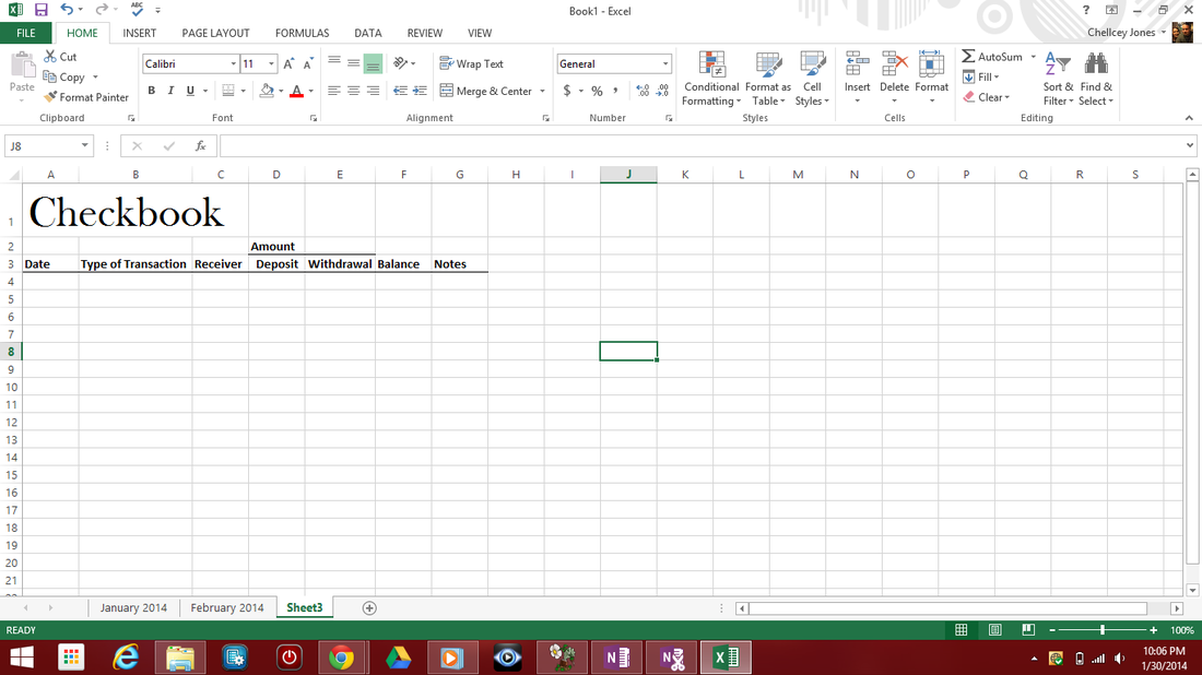
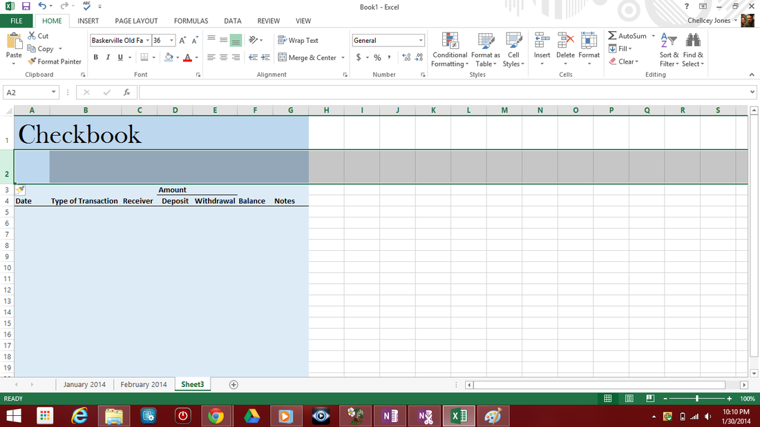
Open Excel and start with a heading and column labels. Here I've titled the sheet "Checkbook" and changed it to a font I liked. The column labels are pretty self-explanatory:
Date, Type of Transaction, Receiver, Deposit, Withdrawal, Balance and Notes with "Amount" above Deposit and Withdrawal.
Let's make our checkbook look a little prettier and more orderly with some colors. First, highlight the heading ("Checkbook").
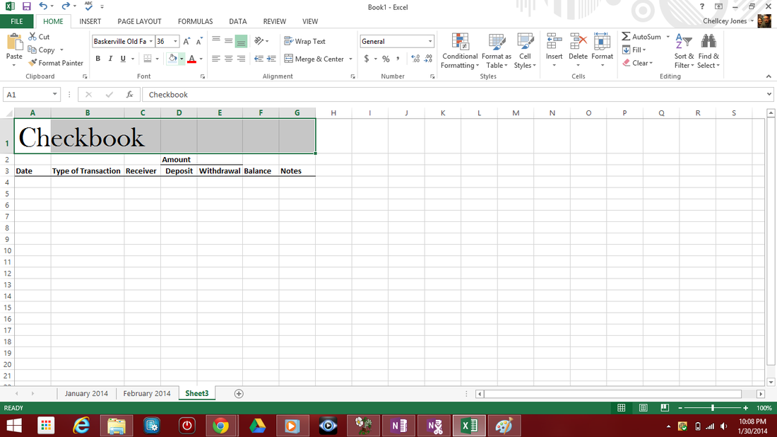
Then click on the paint can and choose a color you like. Generally, the header should be darker than the body (just general rules or formatting... do what pleases you!!).
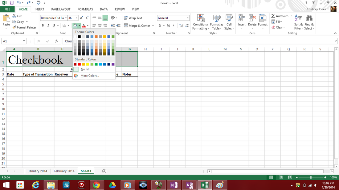
I chose the lightest blue shade for the body and 1 shade darker for the heading.
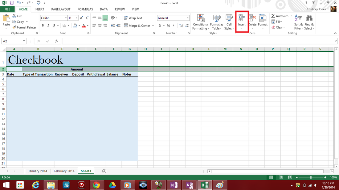
The next step will be adding the month to our checkbook. This will also teach you how to easily insert rows into the spreadsheet.
Select the number of the row that will be BELOW the new row you want to insert. Here, I want the row that has "Amount" in it to be BELOW the month, thus I click the "2" on the left hand side and it highlights the entire row. Next, click "Insert," as shown in the red box below.
Ta-Da! A new row is inserted.
Now, I want to type "January 2014" in the box farthest to the right in our new row. I do so and hit "enter" annnnndddd.....
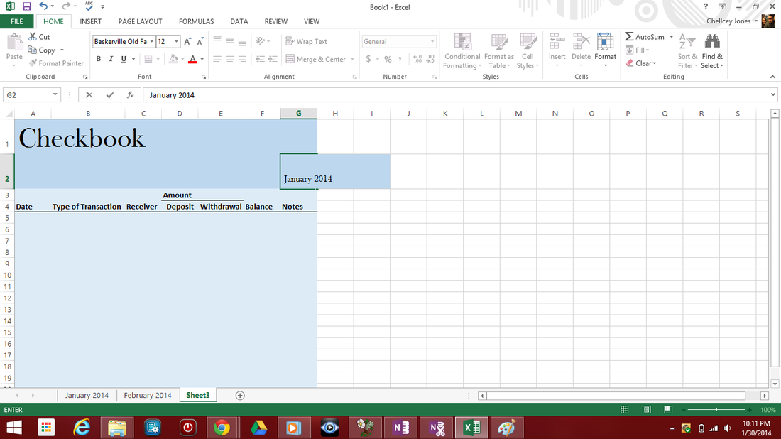
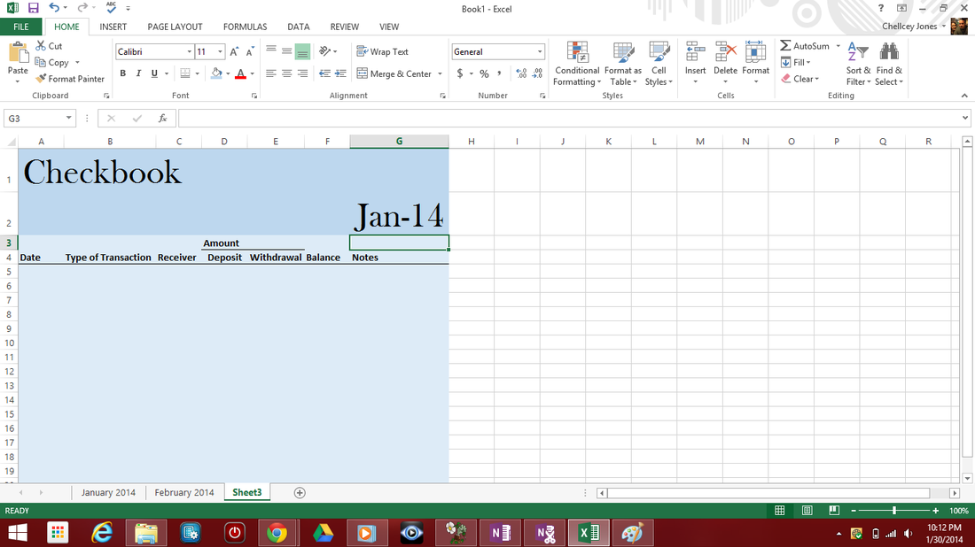
This happens. No matter how many times you type "January 2014," it will keep reverting to this. To stop Excel from doing this, simply put an apostrophe before the text. So, if we type 'January 2014, the apostraophe signals to Excel to override the preset formatting and leaves exactly what we type. Then simply change the font size (I chose size 12).
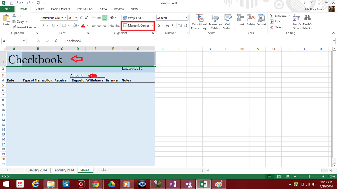
A little more formatting.... Let's "merge and center" our heading and "amount." Highlight "Checkbook" and all the cells that are to be merged. We want the heading to be at the center of our worksheet, so choose cells A1-G1 and hit "Merge and Center" as indicated by the red box below.
Do the same for "Amount," centering the text above the "Deposit" and "Withdrawl" boxes.
Do the same for "Amount," centering the text above the "Deposit" and "Withdrawl" boxes.
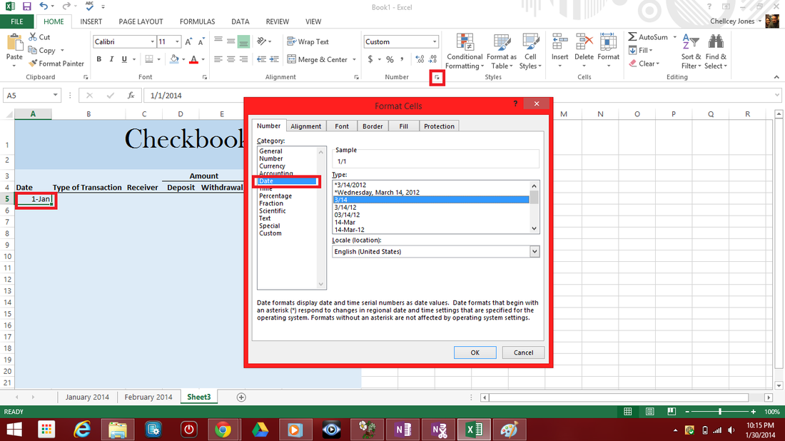
Now let's enter our first date. Typing "01/01" into the first date cell presents us with another Excel formatting override and changes it to "1-Jan." To fix it this time, select the cell with the date and click on the small arrow in the bottom right corner of "Numbers" in the ribbon.
This will bring up a popup up (lol). Click "Date" on the left side and select a date format option that you like. I chose the third option down which makes my date appear "1/1."
This will bring up a popup up (lol). Click "Date" on the left side and select a date format option that you like. I chose the third option down which makes my date appear "1/1."
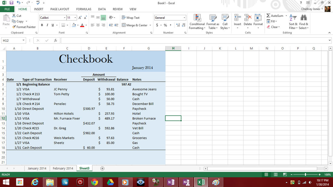
Now let's enter some data. First enter your "Beginning Balance" in the first row. This is the amount of money you have in your account at the beginning of January before spending anything in the month.
Enter the rest of your deposits and withdrawals for the rest of the month as shown below.
Enter the rest of your deposits and withdrawals for the rest of the month as shown below.
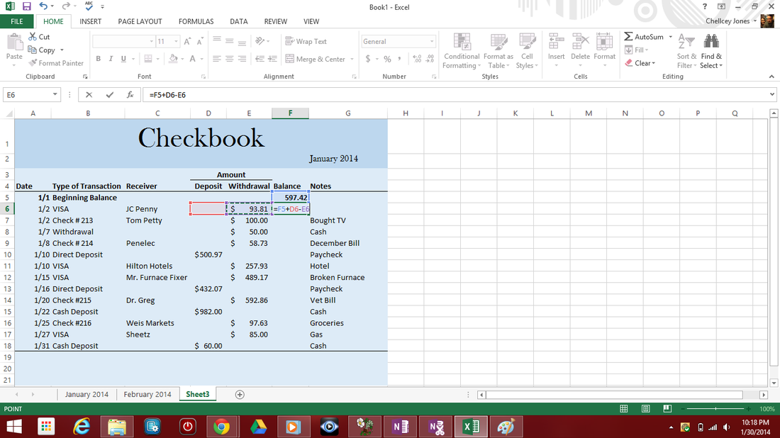
Now on to our first formula! We want our balance to update automatically when we put in a deposit or withdrawal without us having to do anything... Let Excel do the work!
So first, click the empty box below January's beginning balance (F5) and press the = sign. Then click the beginning balance, hit +, then click the deposit box, hit - , and hit the withdrawals box and hit enter. Your formula should read
=F5+D6-D7
And what we have basically done is taken the first balance and added any deposits and subtracted any withdrawals.
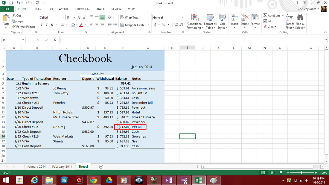
If you put in the same numbers I did, your balance should read as below:
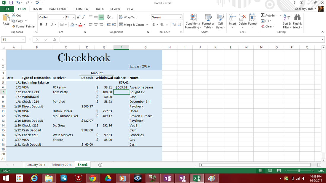
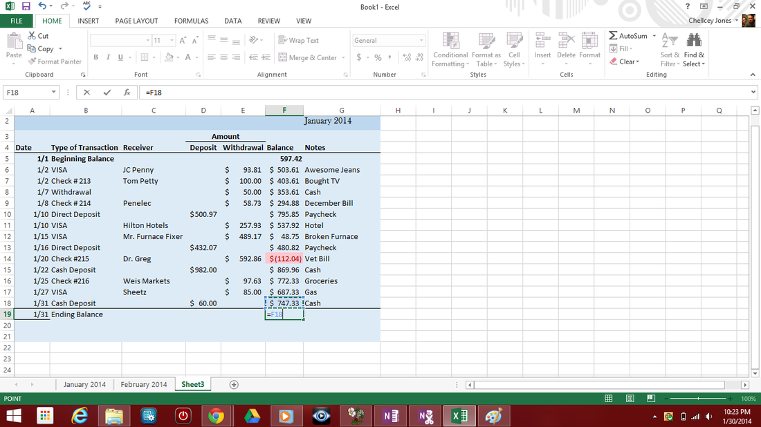
To get all of the balance cells to fill automatically, we have to drag the formula down through them. So click the little square in the bottom right corner of the cell with the formula we just put in and simply drag your curser down to the last balance cell.
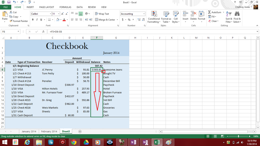
Now all of our balances are filled in. You can simply fix the missing line at the bottom (dragging formulas also drags formatting.... not something we need to really learn about in this how-to).
We also have a negative balance. Wouldn't it be nice if our spreadsheet automatically highlighted our negative balances for us?
We also have a negative balance. Wouldn't it be nice if our spreadsheet automatically highlighted our negative balances for us?
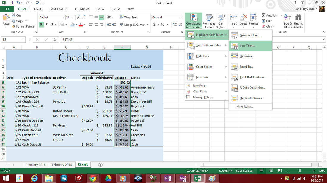
We will use "Condititional Formatting" to do that. Highlight all of the cells in the Balance column.
Click "Conditional Formatting"
Put your mouse over "Highlight Cell Rules"
And then click "Less Than..."
Click "Conditional Formatting"
Put your mouse over "Highlight Cell Rules"
And then click "Less Than..."
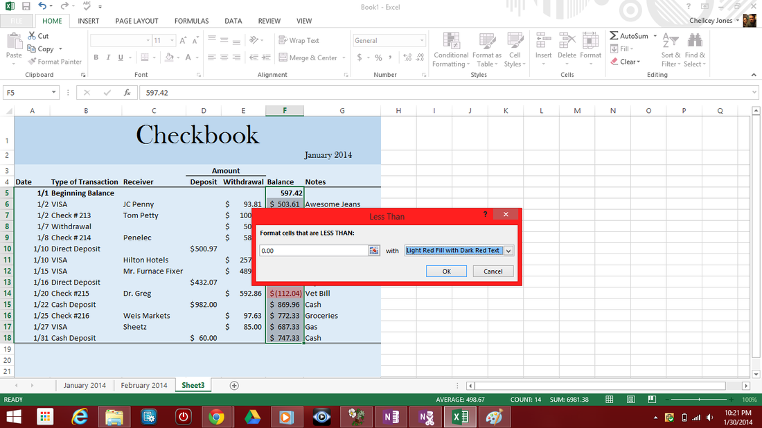
This popup box will appear. Change the amount in the box on the left to "0.00" and click ok.
What we have just done is set a rule so that if any values in the Balance column go below $0.00, that cell will be highlighted red.
You can tailor this any way you want! If you have a rule for your checking account that you don't want the balance to dip below $200, you can do that the same way. Just change the value in the popup box to "200.00" and any value in Balance that goes below $200 will be highlighted red.
Almost done!!
Type in the last date of the month and Ending Balance below your total line. Put an "=" sign in the final Balance cell and have it equal the value above it. You can also put a double underline under the Ending Balance row (it looks nice and is a general accounting practice).
Now we have finished our checkbook! To keep this going monthly, create a new sheet by clicking the "+" along the tabs towards the bottom of the screen. Right-click on the new sheet and click "rename" to put in the name of the month.
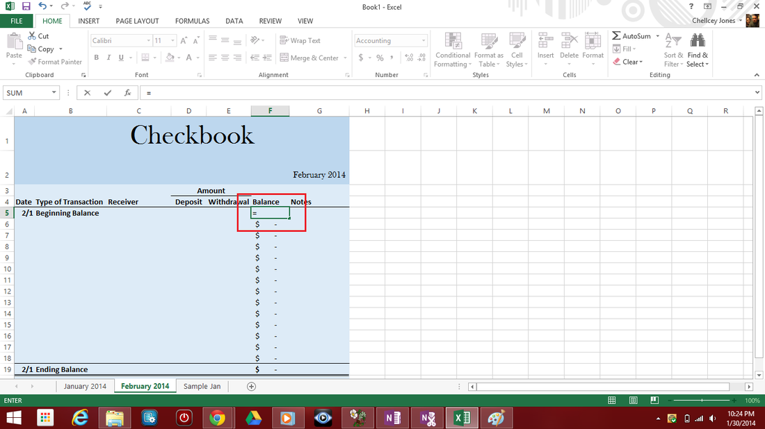
You can then copy and paste everything you just created into the new sheet (this new one would be for February). Simply highlight and delete all the transactions from January and change the month below the heading.
February's beginning balance should equal January's ending balance. So put an "=" sign in the beginning balance for Feb. . . .
February's beginning balance should equal January's ending balance. So put an "=" sign in the beginning balance for Feb. . . .
Click the tab that goes back to the month of January and click on the Ending Balance. Hit "Enter" annnnndddd.......
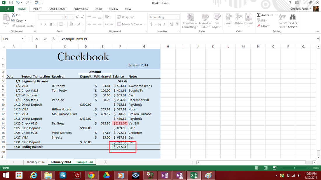
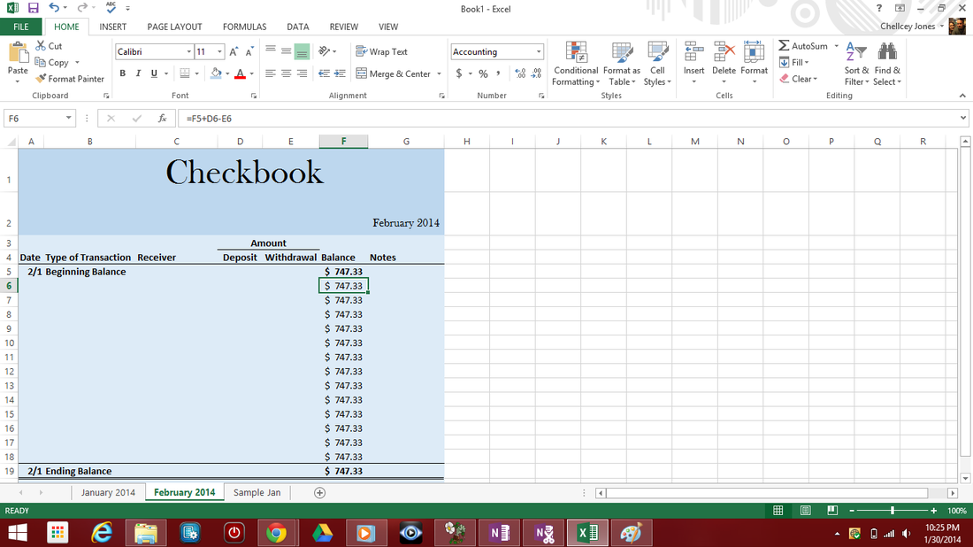
Your screen will jump back to February with the balance filled in. And we are done!! :)
I really hope you found this tutorial useful and helpful!!
If there is an interest, my next tutorial will be using these sheets to do some data analysis to view where our spending goes and how to properly budget.
God Bless
><>
If there is an interest, my next tutorial will be using these sheets to do some data analysis to view where our spending goes and how to properly budget.
God Bless
><>
